Genetic Variant Classification Pr
The Genetic Variant Classification dataset is a sample of observations from the Clinvar archive, which is searchable collection of submissions from medical genetics laboratories and research institutions. Submissions consist of annotations of human genetic variants, and include many measures of the position of variants in the human genome, the type of variants, the likely disease outcome, and disease severity. The dataset used here was created in order to predict whether a variation has conflicting disease-severity classification from different submissions in the Clinvar archive.
Lets take a look at the data!
EDA
def MissingUniqueStatistics(df): #from a kaggle EDA tutorial

  total_entry_list = []
  total_missing_value_list = []
  missing_value_ratio_list = []
  data_type_list = []
  unique_values_list = []
  number_of_unique_values_list = []
  variable_name_list = []

  for col in df.columns:

    variable_name_list.append(col)
    missing_value_ratio = round((df[col].isna().sum()/len(df[col])),4)
    total_entry_list.append(df[col].shape[0] - df[col].isna().sum())
    total_missing_value_list.append(df[col].isna().sum())
    missing_value_ratio_list.append(missing_value_ratio)
    data_type_list.append(df[col].dtype)
    unique_values_list.append(list(df[col].unique()))
    number_of_unique_values_list.append(len(df[col].unique()))

  data_info_df = pd.DataFrame({'Variable':variable_name_list,'#_Total_Entry':total_entry_list,\
                           '#_Missing_Value':total_missing_value_list,'%_Missing_Value':missing_value_ratio_list,\
                           'Data_Type':data_type_list,'Unique_Values':unique_values_list,\
                           '#_Uniques_Values':number_of_unique_values_list})

  return data_info_df.sort_values(by="#_Missing_Value",ascending=False)
df = pd.read_csv(path)
df.shape
(65188, 46)
Below we see a summary table of each column in the dataset. Some things to notice: Most columns names are not meaningful to non-experts. There is wide variety of data encodings, again difficult to interpret. There are many columns with a very high proportion of missing values. There are many high cardinality catagorical columns. On the bright side: There’s alot of data here and some of it looks usable. The summary function was copied from this notebook: https://www.kaggle.com/haliloglumehmet/genetic-variant-classification
MissingUniqueStatistics(df)
| Variable | #_Total_Entry | #_Missing_Value | %_Missing_Value | Data_Type | Unique_Values | #_Uniques_Values | |
|---|---|---|---|---|---|---|---|
| 41 | MOTIF_SCORE_CHANGE | 2 | 65186 | 1.0000 | float64 | [nan, -0.063, -0.097] | 3 |
| 40 | HIGH_INF_POS | 2 | 65186 | 1.0000 | object | [nan, N] | 2 |
| 39 | MOTIF_POS | 2 | 65186 | 1.0000 | float64 | [nan, 1.0] | 2 |
| 38 | MOTIF_NAME | 2 | 65186 | 1.0000 | object | [nan, Egr1:MA0341.1, FOXA1:MA0546.1] | 3 |
| 33 | DISTANCE | 108 | 65080 | 0.9983 | float64 | [nan, 1811.0, 1855.0, 2202.0, 1651.0, 1407.0, ... | 97 |
| 17 | SSR | 130 | 65058 | 0.9980 | float64 | [nan, 1.0, 16.0] | 3 |
| 12 | CLNSIGINCL | 167 | 65021 | 0.9974 | object | [nan, 424754:Likely_pathogenic, 30118:risk_fac... | 138 |
| 8 | CLNDISDBINCL | 167 | 65021 | 0.9974 | object | [nan, MedGen:C1828210,OMIM:153870,Orphanet:ORP... | 94 |
| 10 | CLNDNINCL | 167 | 65021 | 0.9974 | object | [nan, Bull's_eye_maculopathy|Methylmalonic_aci... | 102 |
| 27 | INTRON | 8803 | 56385 | 0.8650 | object | [nan, 6/27, 8/17, 3/20, 24/24, 6/38, 16/38, 20... | 1930 |
| 37 | PolyPhen | 24796 | 40392 | 0.6196 | object | [benign, probably_damaging, nan, possibly_dama... | 5 |
| 36 | SIFT | 24836 | 40352 | 0.6190 | object | [tolerated, deleterious_low_confidence, delete... | 5 |
| 45 | BLOSUM62 | 25593 | 39595 | 0.6074 | float64 | [2.0, -3.0, -1.0, nan, -2.0, 1.0, 3.0] | 7 |
| 14 | CLNVI | 27659 | 37529 | 0.5757 | object | [UniProtKB_(protein):Q96L58#VAR_059317, OMIM_A... | 27655 |
| 35 | BAM_EDIT | 31969 | 33219 | 0.5096 | object | [nan, OK, FAILED] | 3 |
| 32 | Codons | 55184 | 10004 | 0.1535 | object | [gaG/gaC, cCg/cTg, aTc/aCc, Ggc/Agc, Ggc/Tgc, ... | 2221 |
| 31 | Amino_acids | 55184 | 10004 | 0.1535 | object | [E/D, P/L, I/T, G/S, G/C, G/R, S/P, V/M, T/M, ... | 1263 |
| 30 | Protein_position | 55233 | 9955 | 0.1527 | object | [174, 170, 80, 34, 117, 534, 634, 1102, 1225, ... | 7340 |
| 29 | CDS_position | 55233 | 9955 | 0.1527 | object | [522, 509, 239, 100, 349, 1600, 1901, 3304, 36... | 13664 |
| 26 | EXON | 56295 | 8893 | 0.1364 | object | [1/1, 4/4, 6/12, 1/7, 9/17, 15/17, 27/30, 26/3... | 3265 |
| 28 | cDNA_position | 56304 | 8884 | 0.1363 | object | [552, 523, 632, 132, 381, 1858, 2159, 3562, 39... | 13971 |
| 42 | LoFtool | 60975 | 4213 | 0.0646 | float64 | [nan, 0.101, 0.021, 0.0674, 0.183, 0.3, 0.372,... | 1196 |
| 43 | CADD_PHRED | 64096 | 1092 | 0.0168 | float64 | [1.053, 31.0, 28.1, 22.5, 24.7, 23.7, 0.172, 2... | 9325 |
| 44 | CADD_RAW | 64096 | 1092 | 0.0168 | float64 | [-0.208682, 6.517838, 6.061752, 3.114491, 4.76... | 63804 |
| 15 | MC | 64342 | 846 | 0.0130 | object | [SO:0001583|missense_variant, SO:0001583|misse... | 91 |
| 22 | SYMBOL | 65172 | 16 | 0.0002 | object | [B3GALT6, TMEM240, GNB1, SKI, PRDM16, NPHP4, R... | 2329 |
| 25 | BIOTYPE | 65172 | 16 | 0.0002 | object | [protein_coding, misc_RNA, nan] | 3 |
| 34 | STRAND | 65174 | 14 | 0.0002 | float64 | [1.0, -1.0, nan] | 3 |
| 23 | Feature_type | 65174 | 14 | 0.0002 | object | [Transcript, MotifFeature, nan] | 3 |
| 24 | Feature | 65174 | 14 | 0.0002 | object | [NM_080605.3, NM_001114748.1, NM_002074.4, XM_... | 2370 |
| 9 | CLNDN | 65188 | 0 | 0.0000 | object | [not_specified, Spinocerebellar_ataxia_21|not_... | 9260 |
| 2 | REF | 65188 | 0 | 0.0000 | object | [G, A, T, C, CAG, GCCCTCCTCTGAGTCTTCCTCCCCTTCC... | 866 |
| 3 | ALT | 65188 | 0 | 0.0000 | object | [C, A, G, T, CT, TTCC, TA, GGCA, GA, GGAAGAA, ... | 458 |
| 4 | AF_ESP | 65188 | 0 | 0.0000 | float64 | [0.0771, 0.0, 0.1523, 0.0045, 0.0019, 0.0048, ... | 2842 |
| 5 | AF_EXAC | 65188 | 0 | 0.0000 | float64 | [0.1002, 0.0, 1e-05, 0.13103, 0.00357, 0.00231... | 6667 |
| 6 | AF_TGP | 65188 | 0 | 0.0000 | float64 | [0.1066, 0.0, 0.106, 0.003, 0.0058, 0.001, 0.0... | 2087 |
| 7 | CLNDISDB | 65188 | 0 | 0.0000 | object | [MedGen:CN169374, MedGen:C1843891,OMIM:607454,... | 9234 |
| 11 | CLNHGVS | 65188 | 0 | 0.0000 | object | [NC_000001.10:g.1168180G>C, NC_000001.10:g.147... | 65188 |
| 1 | POS | 65188 | 0 | 0.0000 | int64 | [1168180, 1470752, 1737942, 2160305, 2160554, ... | 63115 |
| 13 | CLNVC | 65188 | 0 | 0.0000 | object | [single_nucleotide_variant, Deletion, Duplicat... | 7 |
| 16 | ORIGIN | 65188 | 0 | 0.0000 | int64 | [1, 35, 33, 5, 37, 3, 32, 17, 41, 513, 9, 2, 5... | 31 |
| 18 | CLASS | 65188 | 0 | 0.0000 | int64 | [0, 1] | 2 |
| 19 | Allele | 65188 | 0 | 0.0000 | object | [C, A, G, T, -, TCC, GCA, GAAGAA, GAA, CA, GAG... | 374 |
| 20 | Consequence | 65188 | 0 | 0.0000 | object | [missense_variant, missense_variant&splice_reg... | 48 |
| 21 | IMPACT | 65188 | 0 | 0.0000 | object | [MODERATE, MODIFIER, LOW, HIGH] | 4 |
| 0 | CHROM | 65188 | 0 | 0.0000 | object | [1, 2, 3, 4, 5, 6, 7, 8, 9, 10, 11, 12, 13, 14... | 38 |
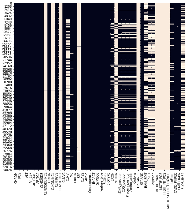
Below we see a plot of missing values for each column in the dataset. Some are completely empty, some very sparse. Other things that caught my eye: Intro/exon look to be inverses of each other, and there is a group of features in the middle-right of the plot that have missing values at the same postions.
fig = plt.figure(figsize = (10, 10))
sns.heatmap(df.isnull(), cbar = False)
<matplotlib.axes._subplots.AxesSubplot at 0x7f14245485e0>
Wrangler
The wrangle function below:
- Determine a unique identfier feature and set it as the dataFrame index
- Drop all columns with greater than 70% missing values
- Drop columns that seem to be redundant or linearly dependent in order to mitigate colinearty problems
- Drop all catagorical columns with cardinality of 1 or greater than 300
- Convert ‘CHROM’, the chromosome id column, from string to integer dtype.
- Remove all rows with missing data.
We go from a 65188 x 46 dataframe to a 59392 x 11 dataframe. The columns now consist of a few genome-positional features, two variant-type feature, and a several impact-prediction scores.
df = pd.read_csv(path)
df.shape
(65188, 46)
def wrangle(df):
    # clean and set CLNHGVS as index
    index_nums = df['CLNHGVS'].apply(lambda x: re.findall(r'\d+', x))
    df['CLNHGVS'] = np.array([lyst[2] for lyst in index_nums.values]).astype('int')
    df.set_index('CLNHGVS', inplace=True)

    #find high-proportion-NaN columns (>.3), drop them.
    ratio_nan = (np.array([df[col].isna().sum() for col in df.columns]) / len(df)).round(3)
    ratio_nans = pd.Series(index=df.columns, data=ratio_nan)
    high_nans = list(ratio_nans.loc[ratio_nans > 0.3].index)
    df.drop(columns=high_nans, inplace=True)

    #Drop 'cDNA_position' & 'Protein_position' : linear-dependent with 'CDS_position'
    df.drop(columns=['cDNA_position','Protein_position'], inplace=True)

    #Find catagorical features with cardinality between 2 and 300 -> low_card_cat_cols list
    cat_cols = df.select_dtypes(include='object').columns
    low_card_cat_cols = []
    for col in cat_cols:
        cardinality = df[col].unique().shape[0]
        if (cardinality < 300) and (cardinality > 1):
            low_card_cat_cols.append(col)

    #numeric features to keep
    num_cols = df.select_dtypes(include='number').columns

    # df composed of low(ish) cardinality catagoricals and numericals
    all_cols = np.concatenate((low_card_cat_cols, num_cols))
    df = df[all_cols]

    #Convert 'CHROM' data points
    df['CHROM'][df['CHROM']=='X'] = 23
    df['CHROM'][df['CHROM']=='MT'] = 24
    df['CHROM'] = df['CHROM'].astype('int')

    df.dropna(inplace=True) ## dropping nan rows 8000 -> 5000 rows, come back if time.

    # BIOTYPE and Feature_type have only 1 value, after dropna() call,
    # Consequence is redundant with MC, CADD_PHRED is redundant with CADD_raw
    # AF_ESP and AF_TGP are redundant with AF_EXAC
    df.drop(columns = ['BIOTYPE', 'Feature_type', 'Consequence', 'CADD_PHRED', 'AF_ESP', 'AF_TGP'], inplace=True)


    return df
df = wrangle(df)
df.shape
(59392, 11)
#take just the first of multiple variant types

df['MC'] = df['MC'].apply(lambda x: x.split('|')[1].split(',')[0])
MissingUniqueStatistics(df)
| Variable | #_Total_Entry | #_Missing_Value | %_Missing_Value | Data_Type | Unique_Values | #_Uniques_Values | |
|---|---|---|---|---|---|---|---|
| 0 | CHROM | 59392 | 0 | 0.0 | int64 | [1, 2, 3, 4, 5, 6, 7, 8, 9, 10, 11, 12, 13, 14... | 23 |
| 1 | CLNVC | 59392 | 0 | 0.0 | object | [single_nucleotide_variant, Deletion, Duplicat... | 7 |
| 2 | MC | 59392 | 0 | 0.0 | object | [missense_variant, splice_donor_variant, synon... | 11 |
| 3 | IMPACT | 59392 | 0 | 0.0 | object | [MODERATE, MODIFIER, LOW, HIGH] | 4 |
| 4 | POS | 59392 | 0 | 0.0 | int64 | [3328358, 3328659, 3347452, 5925304, 5926503, ... | 57704 |
| 5 | AF_EXAC | 59392 | 0 | 0.0 | float64 | [0.0, 0.13103, 0.00357, 0.00231, 0.00267, 0.00... | 6219 |
| 6 | ORIGIN | 59392 | 0 | 0.0 | int64 | [1, 5, 33, 37, 3, 17, 41, 513, 9, 2, 57, 49, 4... | 27 |
| 7 | CLASS | 59392 | 0 | 0.0 | int64 | [0, 1] | 2 |
| 8 | STRAND | 59392 | 0 | 0.0 | float64 | [1.0, -1.0] | 2 |
| 9 | LoFtool | 59392 | 0 | 0.0 | float64 | [0.101, 0.021, 0.0674, 0.183, 0.3, 0.372, 0.27... | 1193 |
| 10 | CADD_RAW | 59392 | 0 | 0.0 | float64 | [-0.543433, 3.424422, 1.126629, 2.96965, 5.430... | 59131 |
Splits
The target for classification in this dataset is pre-determined. The columns ‘CLASS’ is a binary catagory, ‘0’ encodes the agreement, ‘1’ encodes disagreement on the pathogenicity of the varient(row).
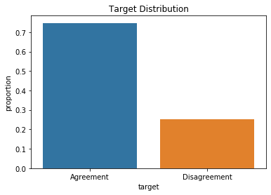
This is an imbalanced target with ~75% / ~25% agreement/disagreement classifications. I use the ‘stratification=y’ kwarg in train_test_split in order to maintain the target distribution in the training and testing sets.
target = 'CLASS'
X = df.drop(columns=target)
y = df[target]
target_dist = y.value_counts(normalize=True).values
ax = sns.barplot(x=['Agreement','Disagreement'], y=target_dist)
ax.set_ylabel('proportion')
ax.set_xlabel('target')
ax.set_title('Target Distribution')
plt.show()
target_dist
array([0.74717134, 0.25282866])
# train-val split, use stratify=y kwarg to maintain class distribution
X_train, X_val, y_train, y_val = train_test_split(X, y, stratify=y, test_size=0.2, random_state=42)
y_val.value_counts(), y_val.value_counts(normalize=True) #verify maintenance of class distribution
(0    8876
 1    3003
 Name: CLASS, dtype: int64,
 0    0.747201
 1    0.252799
 Name: CLASS, dtype: float64)
y_train.value_counts(), y_train.value_counts(normalize=True) #verify maintenance of class distribution
(0    35500
 1    12013
 Name: CLASS, dtype: int64,
 0    0.747164
 1    0.252836
 Name: CLASS, dtype: float64)
Baseline
In our past assignments we have used majority-class-proportion as a baseline for classification models. Due to the target imbalance in this dataset, majority-class-proportion does not tell us much about the predictive power of our classifiers. Accuracy will be high even when classifying randomly. Instead, I choose to use a ROC-AUC score as my baseline, which summarizes true and false positive prediction rates. The worst case is a ROC-AUC score close to 0.5. Perfect predictive power is indicated by ROC-AUC of 1.0.
In order to determine the ROC-AUC score one must fit the training data to some model and make a prediction on the test data. Here I use the sklearn DummyClasifier using the ‘stratified’ strategy, which classifies observations randomly but at the target distribution proportions. As expected, the baseline for this model is an ROC-AUC score of ~0.5.
from sklearn.dummy import DummyClassifier

dummy_clf = DummyClassifier(strategy='stratified')
dummy_clf.fit(X_train, y_train)
y_pred_dummy = dummy_clf.predict(y_val)
# doing lots of ROC plots, so function to save space
def rocplot(model, rows, pos, title):
    y_pred_proba = model.predict_proba(X_val)[:, 1]
    fpr, tpr, threshold = roc_curve(y_val, y_pred_proba)

    plt.subplot(1,rows,pos)
    plt.plot(fpr, tpr)
    plt.plot([0,1], ls='--')
    plt.title(title+' ROC curve')
    plt.xlabel('False Positive Rate')
    plt.ylabel('True Positive Rate')
f = plt.figure(figsize=(5,4))

rocplot(dummy_clf, 1, 1, 'Baseline')

plt.show()
print('Baseline ROC-AUC Score: ', roc_auc_score(y_val, y_pred_dummy))
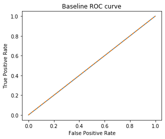
Baseline ROC-AUC Score: 0.496607887380758
Models
Linear Classification: Logistic Regression
In the logistic regression model below we define a preprocessor in order to handle catagorical and numerical features differently. Categorical features are one-hot-encoded, numerical features are scaled to between -1.0 and 1.0.
Again, due to the target imbalance in the data, special precautions are taken in order to mitigate poor performance on the minortiy class. Here I use the ‘SMOTE’ resampler from the ‘imbalanced’ library, which creates new observations of the minority class that are close to the existing ones such that the resampled training set is balanced.
I use sklearn’s RandomizedSearchCV to select an appropriate ‘C’ level for the LogisticRegression classifier.
The best performing model uses a ‘C’ level of 1, and has an ROC-AUC score of 0.582. This is very modestly better than the baseline.
cat_features = ['CHROM', 'CLNVC', 'MC', 'IMPACT'] #catagorical features
cat_transformer = OneHotEncoder(use_cat_names=True) #transformer for cat_features

num_features = ['POS', 'AF_EXAC', 'ORIGIN', 'STRAND', 'LoFtool', 'CADD_RAW'] #numerical features
num_transformer = StandardScaler() #remove mean, scale to between -1 and 1

#column transformer to handle numerical and catagorical features seperately
preprocessor = ColumnTransformer(
    transformers=[
        ('num', num_transformer, num_features),
        ('cat', cat_transformer, cat_features)])

#imbpipeline to accomedate smote, need to encode catagorical features before handing to smote
pipeline = imbpipeline(steps = [['preprocessor', preprocessor],
                                ['smote', SMOTE(random_state=42)],
                                ['classifier', LogisticRegression(random_state=42)]
                               ])

#make folds while preserving target class distribution.(Do I need this given I've already done splits?)
stratified_kfold = StratifiedKFold(n_splits=3)

# 'C' is a regularization parameter, lower numbers enforce higher regularization.
param_grid = {'classifier__C':[0.001, 0.01, 0.1, 1, 10, 100, 1000]}
rand_search = RandomizedSearchCV(pipeline,
                           param_grid,
                           scoring='roc_auc', #scoring by roc_auc since it's my baseline?
                           cv=stratified_kfold,
                           n_jobs=-1)

rand_search.fit(X_train, y_train);
model_LR = rand_search
print('best hyperparameters: ', model_LR.best_params_, '\n')
print('TRAINING ACCURACIES: \n', classification_report(y_train, model_LR.predict(X_train)), '\n')
print('VALIDATION ACCURACIES: \n', classification_report(y_val, model_LR.predict(X_val)))
best hyperparameters:  {'classifier__C': 1}

TRAINING ACCURACIES:
               precision    recall  f1-score   support

           0       0.86      0.30      0.45     35500
           1       0.29      0.86      0.44     12013

    accuracy                           0.44     47513
   macro avg       0.58      0.58      0.44     47513
weighted avg       0.72      0.44      0.45     47513


VALIDATION ACCURACIES:
               precision    recall  f1-score   support

           0       0.86      0.31      0.46      8876
           1       0.30      0.85      0.44      3003

    accuracy                           0.45     11879
   macro avg       0.58      0.58      0.45     11879
weighted avg       0.72      0.45      0.45     11879
Decision Tree Ensemble: Random Forest Classifier
The Random Forest models again uses a ColumnTransformer to handle catagorical and numerical features seperately. Because decision tree classifiers don’t treat catagorical encodings as distances in the way linear regression does, we can use an OrdinalEncoder to maintain dimensionality. Similarly, numerical features do not need to be scaled as they do with linear regression models.
SMOTE is used again to over-sample our minority class and balance the data before handing it to the classifier.
RandomizedSearchCV is used to tune the hyperparameters max-depth, n_estimators, and min_sample_split of RandomForestClassifier.
The best performing model from the cross-validator has a max_depth of 75, n_estimators of 180, and min_sample_split of 9. The ROC-AUC score of 0.657, a modest improvement over the baseline of 0.5.
cat_features = ['CHROM', 'CLNVC', 'MC', 'IMPACT']
cat_transformer = OrdinalEncoder() #use ordinal encoder for decision tree models

num_features = ['POS', 'AF_EXAC', 'ORIGIN', 'STRAND', 'LoFtool', 'CADD_RAW']

preprocessor = ColumnTransformer(
    transformers=[
        ('cat', cat_transformer, cat_features),
        ('num', 'passthrough', num_features) #no scaler for decision tree models
        ])

pipeline = imbpipeline(steps = [['preprocessor', preprocessor],
                                ['smote', SMOTE(random_state=42)],
                                ['classifier', RandomForestClassifier(random_state=42)]
                               ])

stratified_kfold = StratifiedKFold(n_splits=3)

param_grid = {
    'classifier__max_depth': range(50,100,5), #how far each tree extends
    'classifier__n_estimators': range(150,220,10), #number of trees in the forest
    'classifier__min_samples_split': range(2, 10, 1) #min number of samples to form a node
}

rand_search = RandomizedSearchCV(pipeline,
                           param_grid,
                           scoring='roc_auc',
                           cv=stratified_kfold,
                           n_jobs=-1)

rand_search.fit(X_train, y_train);
model_RF = rand_search
print('best hyperparameters: ', model_RF.best_params_, '\n')
print('TRAINING ACCURACIES: \n', classification_report(y_train, model_RF.predict(X_train)), '\n')
print('VALIDATION ACCURACIES: \n', classification_report(y_val, model_RF.predict(X_val)))
best hyperparameters:  {'classifier__n_estimators': 180, 'classifier__min_samples_split': 9, 'classifier__max_depth': 75}

TRAINING ACCURACIES:
               precision    recall  f1-score   support

           0       0.95      0.98      0.96     35500
           1       0.92      0.84      0.88     12013

    accuracy                           0.94     47513
   macro avg       0.93      0.91      0.92     47513
weighted avg       0.94      0.94      0.94     47513


VALIDATION ACCURACIES:
               precision    recall  f1-score   support

           0       0.82      0.85      0.83      8876
           1       0.51      0.47      0.49      3003

    accuracy                           0.75     11879
   macro avg       0.67      0.66      0.66     11879
weighted avg       0.74      0.75      0.75     11879
Decision Tree Ensemble: Gradient Boosted Random Forest Classifier
The gradient boosted random forest classifier model looks identical to the random forest model above with the exception of the paramameters used for hyper-parameter search. Max_depth, n_estimators, learning_rate and col_sample_bytree searched.
The best performing model from the cross-validator has a max_depth of 8, n_estimators of 19, learning_rate of 0.45 and col_sample_bytree of 0.9. The ROC-AUC score of 0.666, is modestly better than the baseline of 0.5, and the best score of the three models fit here.
cat_features = ['CHROM', 'CLNVC', 'MC', 'IMPACT']
cat_transformer = OrdinalEncoder()

num_features = ['POS', 'AF_EXAC', 'ORIGIN', 'STRAND', 'LoFtool', 'CADD_RAW']

preprocessor = ColumnTransformer(
    transformers=[
        ('cat', cat_transformer, cat_features),
        ('num', 'passthrough', num_features)
        ])

pipeline = imbpipeline(steps = [['preprocessor', preprocessor],
                                ['smote', SMOTE(random_state=42)],
                                ['classifier', XGBClassifier(n_jobs=-1, random_state=42)]
                               ])

stratified_kfold = StratifiedKFold(n_splits=3)

param_grid = {
    'classifier__n_estimators': range(8, 20),
    'classifier__max_depth': range(6, 10),
    'classifier__learning_rate': [.01, .2, .3, .4, .45, .5], #size of step in regression?
    'classifier__colsample_bytree': [.7, .8, .9, 1.0] #proportion of columns to sample per tree?
}

rand_search = RandomizedSearchCV(pipeline,
                           param_grid,
                           scoring='roc_auc',
                           cv=stratified_kfold,
                           n_jobs=-1)

rand_search.fit(X_train, y_train);
[23:33:55] WARNING: /tmp/build/80754af9/xgboost-split_1619724447847/work/src/learner.cc:1061: Starting in XGBoost 1.3.0, the default evaluation metric used with the objective 'binary:logistic' was changed from 'error' to 'logloss'. Explicitly set eval_metric if you'd like to restore the old behavior.
model_XBRF = rand_search
print('best hyperparameters: ', model_XBRF.best_params_, '\n')
print('TRAINING ACCURACIES: \n', classification_report(y_train, model_XBRF.predict(X_train)), '\n')
print('VALIDATION ACCURACIES: \n', classification_report(y_val, model_XBRF.predict(X_val)))
best hyperparameters:  {'classifier__n_estimators': 19, 'classifier__max_depth': 8, 'classifier__learning_rate': 0.45, 'classifier__colsample_bytree': 0.9}

TRAINING ACCURACIES:
               precision    recall  f1-score   support

           0       0.86      0.84      0.85     35500
           1       0.56      0.58      0.57     12013

    accuracy                           0.78     47513
   macro avg       0.71      0.71      0.71     47513
weighted avg       0.78      0.78      0.78     47513


VALIDATION ACCURACIES:
               precision    recall  f1-score   support

           0       0.83      0.82      0.82      8876
           1       0.49      0.52      0.50      3003

    accuracy                           0.74     11879
   macro avg       0.66      0.67      0.66     11879
weighted avg       0.75      0.74      0.74     11879
Results and Threshold-Tuning
The logistic regression model with a ROC-AUC score of 0.582 was the worst performer of the three models. The two random forest models performed very similarly. The boosted model edged out the bagging model by only 0.016 for an ROC-AUC score of 0.666. (spooky!)
A comparison of the training and validation classification reports above shows only marginal differences between predictions on training and validation sets and indicates that none of the models were grossly over fit to the training data.
None of these models achieved very good predictive power of the minority class. Given the messy and inconsistent nature of the dataset I am encouraged that any improvement over the baseline was achieved.
f = plt.figure(figsize=(13,4))

rocplot(model_LR.best_estimator_, 3, 1, 'LR')
rocplot(model_RF.best_estimator_, 3, 2, 'RF')
rocplot(model_XBRF.best_estimator_, 3, 3, 'XBRF')
plt.show()

print('Logistic Regression ROC-AUC score:' , roc_auc_score(y_val, model_LR.best_estimator_.predict(X_val)).round(decimals=3))
print('Random Forest ROC-AUC score:' , roc_auc_score(y_val, model_RF.best_estimator_.predict(X_val)).round(decimals=3))
print('Boosted Random Forest ROC-AUC score:' , roc_auc_score(y_val, model_XBRF.best_estimator_.predict(X_val)).round(decimals=3))
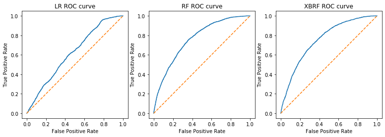
Logistic Regression ROC-AUC score: 0.582
Random Forest ROC-AUC score: 0.657
Boosted Random Forest ROC-AUC score: 0.666
At the suggestion of my instructor (Hi Nivi!), the false-positive-rate(fpr), true-positive-rate(tpr), and threshold for positive classification output by roc_curve() were tabulated. The probability threshold at which tpr ~ 0.75 and fpr ~ 0.4 was found in the table, corresponding to the point on the curve closest to the upper left corner of the plot. That threshold value was 0.26. A new binary prediction was produced by sorting the probability prediction of the XGBoost model as above or below 0.26. Comparing the pre and post threshold-tuned accuracies of the XGboost model predictions, we see a dramatic increase in the recall of the minority(disagreement), at the smaller expense of the precision of the minority. This is an interesting trade-off one can make if precision or recall is preferred.
y_pred_proba = model_XBRF.predict_proba(X_val)[:, 1] #probability predictions by XBRF for X_val

fpr, tpr, thresholds = roc_curve(y_val, y_pred_proba) #roc-curve data saved in variables

roccurve_df = pd.DataFrame({    #throw em in a df
    'False Positive Rate': fpr,
    'True Positive Rate': tpr,
    'Threshold': thresholds
})

roccurve_df[((roccurve_df['False Positive Rate']*10).apply(np.floor) == 4) #query the df for fp~.4, tp~.75
             & ((roccurve_df['True Positive Rate']*10).apply(np.floor) == 8)];
#0.26 at FP ~ 0.4, TP ~ 0.75
y_pred_proba_thresh = y_pred_proba > 0.26
print('PRE-THRESHOLD-TUNED ACCURACIES: \n', classification_report(y_val, model_XBRF.predict(X_val)))
print('POST-THRESHOLD-TUNED ACCURACIES: \n', classification_report(y_val, y_pred_proba_thresh))
PRE-THRESHOLD-TUNED ACCURACIES:
               precision    recall  f1-score   support

           0       0.83      0.82      0.82      8876
           1       0.49      0.52      0.50      3003

    accuracy                           0.74     11879
   macro avg       0.66      0.67      0.66     11879
weighted avg       0.75      0.74      0.74     11879

POST-THRESHOLD-TUNED ACCURACIES:
               precision    recall  f1-score   support

           0       0.89      0.57      0.70      8876
           1       0.39      0.80      0.52      3003

    accuracy                           0.63     11879
   macro avg       0.64      0.68      0.61     11879
weighted avg       0.76      0.63      0.65     11879
Feature Importance
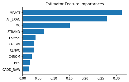
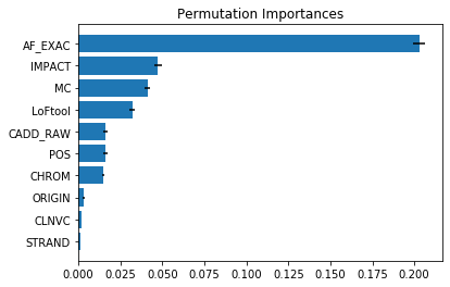
If the models above achieved robust accuracy, it would be of interest to researchers and clinicians which of the features used to predict disagreement are strongest. My models were not very predictive, so the feature importance ranking and metrics below are to be taken very lightly.
The feature importances from the XGBoost model rank ‘AF_EXAC’ as strongest. ‘IMPACT’ is a close second. Both of these features are pathogenicity scores, so it makes sense that they would be predictive. ‘MC’ column comes in a distant third. This feature represents type of variant in the mRNA created from the DNA variant. Given that it has some predictive power, it may be of interest to researchers. All other features make marginal contributions.
Permutation importances show ‘AF-EXAC’ as dominating all other features.
importances =  model_XBRF.best_estimator_.named_steps.classifier.feature_importances_
feature_names = X_train.columns
feat_imp =pd.Series(data=importances,index=feature_names).sort_values()
plt.barh(feat_imp.index, feat_imp.values)
plt.title('Estimator Feature Importances')
plt.show()
perm_imp = permutation_importance(model_XBRF,X_val,y_val,random_state=42)
permutation_importances = pd.DataFrame({'mean_imp': perm_imp['importances_mean'],
                                        'std_imp': perm_imp['importances_std']},
                                        index = X_val.columns).sort_values(by='mean_imp', ascending=False)

plt.barh(permutation_importances.index[-1::-1],
         permutation_importances.mean_imp.sort_values(),
         xerr=permutation_importances.std_imp.sort_values())
plt.title('Permutation Importances')
plt.show()
Informal Discussion
This was a difficult dataset for a novice in both data-science and genetics. My suspicion is that this is primarily a feature engineering problem for which I have neither the skill nor domain-knowledge to really tackle.
Despite the inherent difficulty, I am encouraged to have made a very modestly predictive model. (Although somewhat discouraged to find out at the end that the dominant features were pathogenicity scores). I believe I was successful in following good data-leakage, imbalanced-data-splitting, and hyper-parameter tuning practices. I am not very confident I implemented the SMOTE over-sampling function correctly, I had difficulty finding good usage examples for including catagorical data. There are a number of encoding options, and over/under sampling techniques that I would love to explore given time and compute. I really loved looking into the genetics terminology, and I consider this a first, faltering step of many into this sub-field of data-science.